DACON 가스공급량 수요예측 모델개발

지난 10월 부터 12월까지 진행되었던 Dacon 가스 공급량 수요예측 모델개발 대회의 코드를 공유합니다.

가스공급량이 주로 기온에 영향을 많이 받는 것으로 생각되어 기상청 (https://data.kma.go.kr/cmmn/main.do) 에서 날씨정보를 시간별로 받아 왔고, LNG 가스가 발전에도 사용되기 때문에 전력소비계수도 데이터에 포함 시켰습니다.

최근 들어 늘어난 신재생에너지 발전비율에 따라 시간당 태양광 발전 현황도 가스 사용량에 영향을 미칠 것이라 생각되어 해당 데이터도 포함 시켰습니다.

import os
import pandas as pd
import numpy as np

import seaborn as sns
import matplotlib.pyplot as plt

import warnings 
warnings.filterwarnings('ignore')

from datetime import timedelta

base_path = os.getcwd()

Test dataset 정리

train = pd.read_csv(os.path.join(base_path,"한국가스공사_시간별 공급량_20181231.csv"), encoding='CP949')
test = pd.read_csv(os.path.join(base_path,"test.csv"))

test['연월일'] = test['일자|시간|구분'].str.split(' ').apply(lambda x:x[0])
test['시간'] = test['일자|시간|구분'].str.split(' ').apply(lambda x:x[1])
test['구분'] = test['일자|시간|구분'].str.split(' ').apply(lambda x:x[2])

test.drop('일자|시간|구분',axis=1, inplace=True)

Train/Test dataset 병합

len_train = train.shape[0]

df = pd.concat([train,test])

df['연월일'] = pd.to_datetime(df['연월일'])

df['연'] = df['연월일'].dt.year
df['일'] = df['연월일'].dt.day
df['월'] = df['연월일'].dt.month
df['요일'] = df['연월일'].dt.dayofweek

df['주말'] = df['요일'].apply(lambda x:1 if x == 5 or x==6 else 0)

df['시간'] = df['시간'].astype('int')

df.loc[df['시간']==24,'시간'] = 0
df.loc[df['시간']==0,'연월일'] = df.loc[df['시간']==0,'연월일'].apply(lambda x:x + timedelta(days=1))

from sklearn.preprocessing import LabelEncoder
encoder = LabelEncoder()
df['구분'] = encoder.fit_transform(df['구분'])

Train/Test 분리

train = df[:len_train]
test = df[len_train:]

Train 데이터셋 데이터 추가

from IPython.display import Image
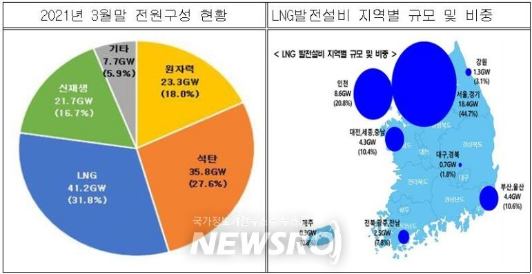
Image(url = "https://www.newsro.kr/wp-content/uploads/2021/05/2021-05-13-171309-771x397.jpeg")

• LNG는 주로 난방 or 발전에 사용됨.

• 난방에 사용되는 LNG의 양은 날씨의 영향을 받고 날씨의 변화는 전국적으로 비슷함.

• 신재생 에너지 발전량이 줄어들면 LNG 발전소의 발전량이 증가함.

• LNG 발전설비는 수도권에 집중되어 있음.

• 날씨 데이터는 서울시 데이터를 사용.

날씨 데이터

weather = pd.read_csv(os.path.join(base_path,"weather", ''.join(["날씨정보", '2013' ,".csv"])), encoding='CP949')
for i in range(2014, 2019):
    weather_data = pd.read_csv(os.path.join(base_path,"weather", ''.join(["날씨정보", str(i) ,".csv"])), encoding='CP949')
    weather = pd.concat([weather, weather_data])

weather.drop(['강수량(mm)', '풍속(m/s)', '습도(%)'], axis=1, inplace=True)

weather = weather.set_axis(['지점', '지점명', '일시', '기온', '증기압', '이슬점온도', '현지기압', '해면기압', '지면온도'],axis=1)

weather['연월일'] = weather['일시'].str.split(' ').apply(lambda x:x[0])
weather['시간'] = weather['일시'].str.split(' ').apply(lambda x:x[1])
weather['시간'] = weather['시간'].apply(lambda x:x[:2]).astype('int')
weather['연월일'] = pd.to_datetime(weather['연월일'])

weather = weather.reset_index().drop(0, axis=0)

train['연월일시'] = train['연월일'].astype('str').str.cat(' '+ train['시간'].astype('str')+':00')

weather['연월일시'] = weather['연월일'].astype('str').str.cat(' '+ weather['시간'].astype('str')+':00')

weather = weather[['연월일시','기온', '증기압', '이슬점온도', '현지기압', '해면기압', '지면온도']]

train = pd.merge(train,weather, on='연월일시', how='left')

전력소비계수(2018)

elec = pd.read_csv(os.path.join(base_path,'GasStatistics','주택용_월별_124시_전력소비계수_2018.csv'), encoding='CP949')

elec.columns = ['월', 1,2,3,4,5,6,7,8,9,10,11,12]

elec.iloc[0,:] = elec.iloc[24,:]

train['전력사용량'] = train.apply(lambda x:elec.iloc[x.시간, x.월], axis='columns')
train['전력사용량'] = train['전력사용량'].astype('int')

태양광 발전 현황(2018)

sun_gen = pd.read_csv(os.path.join(base_path,'GasStatistics','태양광 발전량_2018.csv'), encoding='CP949')
sun_gen = sun_gen.groupby(['거래일', '시간'])[['전력거래량']].sum().reset_index()
sun_gen['거래일'] = pd.to_datetime(sun_gen['거래일'])
sun_gen['월'] = sun_gen['거래일'].dt.month
sun_gen = sun_gen.groupby(['월','시간'])[['전력거래량']].mean().reset_index()

for i in train['월'].unique():
    for j in train['시간'].unique():
        train.loc[(train['월']==i)&(train['시간']==j),'태양광발전량'] = sun_gen.loc[(sun_gen['월']==i)&(sun_gen['시간']==j),'전력거래량'].values[0]

결측치 처리

train.shape

(368088, 18)

train.isnull().sum()

연월일         0
시간          0
구분          0
공급량         0
연           0
일           0
월           0
요일          0
주말          0
연월일시        0
기온         49
증기압        91
이슬점온도     217
현지기압      406
해면기압       42
지면온도      406
전력사용량       0
태양광발전량      0
dtype: int64

for i,j in enumerate(train.columns):
    print(i,j)

0 연월일
1 시간
2 구분
3 공급량
4 연
5 일
6 월
7 요일
8 주말
9 연월일시
10 기온
11 증기압
12 이슬점온도
13 현지기압
14 해면기압
15 지면온도
16 전력사용량
17 태양광발전량

기온

temp_nan_index = train.loc[train['기온'].isnull()==True,'연월일시'].index

# 데이터가 비었을 경우 전시간 데이터로 채워줌.
for i in temp_nan_index:
    j = i-1
    while True:
        if np.isnan(train.iloc[j,10])==False:
            train.iloc[i,10] = train.iloc[j,10]
            break
        else:
            j=j-1

기타 날씨

press_nan_index = train.loc[train['현지기압'].isnull()==True,'연월일시'].index

for i in press_nan_index:
    j = i-1
    while True:
        if np.isnan(train.iloc[j,13])==False:
            train.iloc[i,13] = train.iloc[j,16]
            break
        else:
            j=j-1

vapor_pres = train.loc[train['증기압'].isnull()==True,'연월일시'].index

for i in vapor_pres:
    j = i-1
    while True:
        if np.isnan(train.iloc[j,11])==False:
            train.iloc[i,11] = train.iloc[j,11]
            break
        else:
            j=j-1

dew_point = train.loc[train['이슬점온도'].isnull()==True,'연월일시'].index

for i in dew_point:
    j = i-1
    while True:
        if np.isnan(train.iloc[j,12])==False:
            train.iloc[i,12] = train.iloc[j,12]
            break
        else:
            j=j-1

sea_press = train.loc[train['해면기압'].isnull()==True,'연월일시'].index

for i in sea_press:
    j = i-1
    while True:
        if np.isnan(train.iloc[j,14])==False:
            train.iloc[i,14] = train.iloc[j,14]
            break
        else:
            j=j-1

ground_temp = train.loc[train['지면온도'].isnull()==True,'연월일시'].index

for i in ground_temp:
    j = i-1
    while True:
        if np.isnan(train.iloc[j,15])==False:
            train.iloc[i,15] = train.iloc[j,15]
            break
        else:
            j=j-1

train.isnull().sum()

연월일       0
시간        0
구분        0
공급량       0
연         0
일         0
월         0
요일        0
주말        0
연월일시      0
기온        0
증기압       0
이슬점온도     0
현지기압      0
해면기압      0
지면온도      0
전력사용량     0
태양광발전량    0
dtype: int64

Test set에도 동일 Data 추가

• 날씨의 경우에는 월별 시간 별 평균으로 처리

train

	연월일	시간	구분	공급량	연	일	월	요일	주말	연월일시	기온	증기압	이슬점온도	현지기압	해면기압	지면온도	전력사용량	태양광발전량
0	2013-01-01	1	0	2497.129	2013	1	1	1	0	2013-01-01 1:00	-8.5	1.8	-15.5	1010.0	1021.2	-3.4	951	2.052781
1	2013-01-01	2	0	2363.265	2013	1	1	1	0	2013-01-01 2:00	-8.4	2.0	-14.7	1009.4	1020.6	-3.4	845	0.816043
2	2013-01-01	3	0	2258.505	2013	1	1	1	0	2013-01-01 3:00	-8.1	1.9	-14.9	1009.2	1020.4	-3.4	786	0.193692
3	2013-01-01	4	0	2243.969	2013	1	1	1	0	2013-01-01 4:00	-8.2	1.9	-15.0	1008.2	1019.4	-3.4	761	0.218934
4	2013-01-01	5	0	2344.105	2013	1	1	1	0	2013-01-01 5:00	-8.2	2.0	-14.4	1007.3	1018.5	-3.3	758	0.324555
...	...	...	...	...	...	...	...	...	...	...	...	...	...	...	...	...	...	...
368083	2018-12-31	20	6	681.033	2018	31	12	0	0	2018-12-31 20:00	-3.7	1.8	-15.6	1024.9	1036.1	-3.0	1294	253.693707
368084	2018-12-31	21	6	669.961	2018	31	12	0	0	2018-12-31 21:00	-4.6	1.9	-15.0	1024.8	1036.0	-4.1	1295	121.694997
368085	2018-12-31	22	6	657.941	2018	31	12	0	0	2018-12-31 22:00	-5.4	1.9	-15.2	1024.4	1035.6	-5.0	1277	43.376048
368086	2018-12-31	23	6	610.953	2018	31	12	0	0	2018-12-31 23:00	-5.2	2.0	-14.7	1024.6	1035.8	-5.1	1207	13.010598
368087	2019-01-01	0	6	560.896	2018	31	12	0	0	2019-01-01 0:00	-5.2	2.0	-14.7	1207.0	1035.8	-5.1	1092	9.462802

368088 rows × 18 columns

EDA

sns.boxplot(x='월', y='기온', data=train.loc[(train['구분']==0)])

<AxesSubplot:xlabel='월', ylabel='기온'>

np.array(train.loc[(train['구분']==0)&(train['연']==2014)]['기온'][:2160])

array([ 2.6,  1.7,  1.4, ..., 13.2, 12.5, 12.3])

plt.plot(np.array(train.loc[(train['구분']==0)&(train['연']==2013)]['기온'][:2160]),label='2013')
plt.plot(np.array(train.loc[(train['구분']==0)&(train['연']==2014)]['기온'][:2160]),label='2014')
plt.plot(np.array(train.loc[(train['구분']==0)&(train['연']==2015)]['기온'][:2160]),label='2015')
plt.plot(np.array(train.loc[(train['구분']==0)&(train['연']==2016)]['기온'][:2160]),label='2016')
plt.plot(np.array(train.loc[(train['구분']==0)&(train['연']==2017)]['기온'][:2160]),label='2017')
plt.plot(np.array(train.loc[(train['구분']==0)&(train['연']==2018)]['기온'][:2160]),label='2018')
plt.legend(loc='upper left')

plt.show()

# Outlier 제거 함수

def get_outlier(df=None, column=None, weight=1.5):
    quantile_25 = np.percentile(df[column].values, 25)
    quantile_75 = np.percentile(df[column].values, 75)

    IQR = quantile_75 - quantile_25
    IQR_weight = IQR*weight
  
    lowest = quantile_25 - IQR_weight
    highest = quantile_75 + IQR_weight
  
    outlier_idx = df[column][ (df[column] < lowest) | (df[column] > highest) ].index
    return outlier_idx

sns.boxplot(x='시간', y='기온', data=train.loc[(train['구분']==0)&(train['월']==1)])

<AxesSubplot:xlabel='시간', ylabel='기온'>

sns.boxplot(x='시간', y='기온', data=train.loc[(train['구분']==0)&(train['월']==2)])

<AxesSubplot:xlabel='시간', ylabel='기온'>

sns.boxplot(x='시간', y='기온', data=train.loc[(train['구분']==0)&(train['월']==3)])

<AxesSubplot:xlabel='시간', ylabel='기온'>

mean_train = train[train['구분']==0]

mean_train.drop(get_outlier(mean_train.loc[train['월']==1],'기온'),inplace=True)
mean_train.reset_index(drop=True, inplace=True)
mean_train.drop(get_outlier(mean_train.loc[train['월']==2],'기온'),inplace=True)
mean_train.reset_index(drop=True, inplace=True)
mean_train.drop(get_outlier(mean_train.loc[train['월']==3],'기온'),inplace=True)
mean_train.reset_index(drop=True, inplace=True)

temp_mon_mean = mean_train.groupby(['월','시간'])[['기온', '증기압', 
                                           '이슬점온도', '현지기압', '해면기압', '지면온도', 
                                           '전력사용량', '태양광발전량']].mean().reset_index()

test['기온'] = 0
test['이슬점온도'] = 0
test['현지기압'] = 0
test['해면기압'] = 0
test['지면온도'] = 0
test['태양광발전량'] = 0

for i in test['월'].unique():
    for j in test['시간'].unique():
        test.loc[(test['월']==i)&(test['시간']==j),'기온'] = temp_mon_mean.loc[(temp_mon_mean['월']==i)&(temp_mon_mean['시간']==j),'기온'].values[0]
        test.loc[(test['월']==i)&(test['시간']==j),'증기압'] = temp_mon_mean.loc[(temp_mon_mean['월']==i)&(temp_mon_mean['시간']==j),'증기압'].values[0]
        test.loc[(test['월']==i)&(test['시간']==j),'이슬점온도'] = temp_mon_mean.loc[(temp_mon_mean['월']==i)&(temp_mon_mean['시간']==j),'이슬점온도'].values[0]
        test.loc[(test['월']==i)&(test['시간']==j),'현지기압'] = temp_mon_mean.loc[(temp_mon_mean['월']==i)&(temp_mon_mean['시간']==j),'현지기압'].values[0]
        test.loc[(test['월']==i)&(test['시간']==j),'해면기압'] = temp_mon_mean.loc[(temp_mon_mean['월']==i)&(temp_mon_mean['시간']==j),'해면기압'].values[0]
        test.loc[(test['월']==i)&(test['시간']==j),'지면온도'] = temp_mon_mean.loc[(temp_mon_mean['월']==i)&(temp_mon_mean['시간']==j),'지면온도'].values[0]
        test.loc[(test['월']==i)&(test['시간']==j),'태양광발전량'] = temp_mon_mean.loc[(temp_mon_mean['월']==i)&(temp_mon_mean['시간']==j),'태양광발전량'].values[0]

• test dataset의 전력사용량은 2018년도 Data로 fill up

test['전력사용량'] = test.apply(lambda x:elec.iloc[x.시간, x.월], axis='columns')
test['전력사용량'] = test['전력사용량'].astype('int')

test['연월일시'] = test['연월일'].astype('str').str.cat(' '+ test['시간'].astype('str')+':00')

train['연월일시'] = pd.to_datetime(train['연월일시'])
test['연월일시'] = pd.to_datetime(test['연월일시'])

from workalendar.asia import SouthKorea

train['연월일'] = pd.to_datetime(train['연월일'])

holidays = pd.concat([pd.Series(np.array(SouthKorea().holidays(2013))[:, 0]), pd.Series(np.array(SouthKorea().holidays(2014))[:, 0]), 
           pd.Series(np.array(SouthKorea().holidays(2015))[:, 0]), pd.Series(np.array(SouthKorea().holidays(2016))[:, 0]),
           pd.Series(np.array(SouthKorea().holidays(2017))[:, 0]), pd.Series(np.array(SouthKorea().holidays(2018))[:, 0])]).reset_index(drop=True)

train['is_holiday'] = train['연월일'].dt.date.isin(holidays).astype('int')

test['연월일'] = pd.to_datetime(test['연월일'])

test_holidays = pd.Series(np.array(SouthKorea().holidays(2019))[:, 0]).reset_index(drop=True)

test['is_holiday'] = test['연월일'].dt.date.isin(test_holidays).astype('int')

train_copy = train.copy()
test_copy = test.copy()

train = train_copy
test = test_copy

Outlier 제거

f, ax = plt.subplots(2,3,figsize=(10,10))

ax[0][0].plot(train.loc[(train['구분']==2)&(train['연']==2013)]['공급량'])
ax[0][1].plot(train.loc[(train['구분']==2)&(train['연']==2014)]['공급량'])
ax[0][2].plot(train.loc[(train['구분']==2)&(train['연']==2015)]['공급량'])
ax[1][0].plot(train.loc[(train['구분']==2)&(train['연']==2016)]['공급량'])
ax[1][1].plot(train.loc[(train['구분']==2)&(train['연']==2017)]['공급량'])
ax[1][2].plot(train.loc[(train['구분']==2)&(train['연']==2018)]['공급량'])

plt.show()

• 구분2의 경우 가스공급이 끊기는 경우가 매년 있음.

train.drop(train.loc[(train['공급량']<5)&(train['구분']==2)].index, axis=0, inplace=True)
train.drop(train.loc[(train['공급량']<50)&(train['구분']==2)&(train['연']==2016)].index, axis=0, inplace=True)
train.drop(train.loc[(train['공급량']<50)&(train['구분']==2)&(train['연']==2017)].index, axis=0, inplace=True)
train.drop(train.loc[(train['공급량']<20)&(train['구분']==2)&(train['연']==2018)].index, axis=0, inplace=True)

def get_outlier(df=None, column=None, weight=1.5):
  # target 값과 상관관계가 높은 열을 우선적으로 진행
    quantile_25 = np.percentile(df[column].values, 25)
    quantile_75 = np.percentile(df[column].values, 75)

    IQR = quantile_75 - quantile_25
    IQR_weight = IQR*weight
  
    lowest = quantile_25 - IQR_weight
    highest = quantile_75 + IQR_weight
  
    outlier_idx = df[column][ (df[column] < lowest) | (df[column] > highest) ].index
    return outlier_idx

ax= sns.boxplot(x='구분', y = '공급량', data=train)

train[(train['구분']==0)&(train['공급량']>10000)].index

train.drop(train[(train['구분']==0)&(train['공급량']>10000)].index,inplace=True)

train.drop(train[(train['구분']==5)&(train['공급량']>7000)].index,inplace=True)

train.drop(train[(train['구분']==6)&(train['공급량']>1000)].index,inplace=True)

ax= sns.boxplot(x='구분', y = '공급량', data=train)

상관관계분석

sns.heatmap(train.corr(), annot=True)
plt.gcf().set_size_inches(15, 8)

모델링

SEED = 123

from sklearn.model_selection import train_test_split

from sklearn.tree import DecisionTreeRegressor
from sklearn.ensemble import RandomForestRegressor
from lightgbm import LGBMRegressor
from xgboost import XGBRegressor
from sklearn.neighbors import KNeighborsRegressor

model_dict = {'DT':DecisionTreeRegressor(),
#              'RF':RandomForestRegressor(),
              'LGBM':LGBMRegressor(),
              'XGB':XGBRegressor(),
              'KNN':KNeighborsRegressor()
             }

columns = [
#     '연월일', 
    '시간', 
#     '구분', 
#     '공급량', 
#     '연', 
#     '일', 
    '월', 
    '요일', 
    '주말', 
#     '연월일시', 
    '기온',
    '증기압', 
    '이슬점온도', 
    '현지기압', 
    '해면기압', 
    '지면온도', 
    '전력사용량', 
    'is_holiday',
    '태양광발전량'
]

from sklearn.model_selection import KFold
from sklearn.model_selection import cross_val_score
k_fold = KFold(n_splits=5, shuffle=True, random_state=SEED)
score = {}

for model_name in model_dict.keys():
    model = model_dict[model_name]
    score[model_name] = np.mean(cross_val_score(model, train[columns], train['공급량'], scoring='neg_mean_squared_error', cv=k_fold))
    print(f'{model_name} 평가 완료')

score

DT 평가 완료
LGBM 평가 완료
XGB 평가 완료
KNN 평가 완료

{'DT': -741902.3487673458,
 'LGBM': -535743.8450095323,
 'XGB': -559576.4150579236,
 'KNN': -724182.1721817076}

• Train Set 으로 평가 했을 떄는 LGBM이 점수가 더 잘 나왔지만, 제출시 점수는 XGB가 더 높아서 XGB를 모델로 채택

def nmae(true_df, pred_df):
    true_df = pd.DataFrame(true_df).reset_index()
    pred_df = pd.DataFrame(pred_df).reset_index()

#     nmae 함수를 사용하기 위해 Index Column 통일
    pred_df['index'] = true_df['index']
    target_idx = true_df.iloc[:,0]
    pred_df = pred_df[pred_df.iloc[:,0].isin(target_idx)]
    pred_df = pred_df.sort_values(by=[pred_df.columns[0]], ascending=[True])
    true_df = true_df.sort_values(by=[true_df.columns[0]], ascending=[True])
    
    true = true_df.iloc[:,1].to_numpy()
    pred = pred_df.iloc[:,1].to_numpy()

    score = np.mean((np.abs(true-pred))/true)
    
    return score

train.columns

Index(['연월일', '시간', '구분', '공급량', '연', '일', '월', '요일', '주말', '연월일시', '기온',
       '증기압', '이슬점온도', '현지기압', '해면기압', '지면온도', '전력사용량', '태양광발전량',
       'is_holiday'],
      dtype='object')

from sklearn.preprocessing import MinMaxScaler

scaler = MinMaxScaler()

scaler.fit(train[['기온',
      '증기압', 
    '이슬점온도', 
    '현지기압', 
    '해면기압', 
    '지면온도', 
     '전력사용량',
    '태양광발전량'
     ]])

MinMaxScaler()

train[['기온',
      '증기압', 
    '이슬점온도', 
    '현지기압', 
    '해면기압', 
    '지면온도', 
     '전력사용량',
    '태양광발전량'  
     ]] = scaler.transform(train[['기온',
      '증기압', 
    '이슬점온도', 
    '현지기압', 
    '해면기압', 
    '지면온도', 
     '전력사용량',
    '태양광발전량'   
     ]])

test[['기온',
      '증기압', 
    '이슬점온도', 
    '현지기압', 
    '해면기압', 
    '지면온도', 
     '전력사용량',
    '태양광발전량'
     ]] = scaler.transform(test[['기온',
      '증기압', 
    '이슬점온도', 
    '현지기압', 
    '해면기압', 
    '지면온도', 
     '전력사용량',
    '태양광발전량'
     ]])

xgb_total_score = 0
y_test_arr = np.zeros(shape=(0,))
xgb_arr = np.zeros(shape=(0,))
for i in train['구분'].unique():
#     x_train, x_test, y_train, y_test = train_test_split(train.loc[train['구분']==i,columns], train.loc[train['구분']==i,'공급량'], random_state = SEED)
    x_train = train.loc[(train['연']!=2018)&(train['구분']==i)][columns]
    y_train = train.loc[(train['연']!=2018)&(train['구분']==i)]['공급량']
    x_test = train.loc[(train['연']==2018)&(train['구분']==i)][columns]
    y_test = train.loc[(train['연']==2018)&(train['구분']==i)]['공급량']
    
    y_test_arr = np.append(y_test_arr, y_test)    
    
    xgb = XGBRegressor()
    xgb.fit(x_train, y_train)
    xgb_pred = xgb.predict(x_test)
    xgb_arr = np.append(xgb_arr, xgb_pred)
    score = nmae(y_test, xgb_pred)
    print(f'구분 : {i} 일 때, nmae : {score}')
    xgb_total_score += score
print(f'XGB score 평균: {xgb_total_score/7}')

구분 : 0 일 때, nmae : 0.07251945473552061
구분 : 1 일 때, nmae : 0.08449827175009314
구분 : 2 일 때, nmae : 0.14485647005844865
구분 : 3 일 때, nmae : 0.08794345376682498
구분 : 4 일 때, nmae : 0.10510043321254962
구분 : 5 일 때, nmae : 0.11193264357901477
구분 : 6 일 때, nmae : 0.07871132644407625
XGB score 평균: 0.09793743622093258

• 2018년을 모델 평가 데이터 셋으로 사용

# 구분별로 학습모델을 따로 만들어 학습
sub_xgb = XGBRegressor()
sub_xgb.fit(train.loc[train['구분']==0, columns], train.loc[train['구분']==0,'공급량'])
sub_xgb_pred = sub_xgb.predict(test.loc[test['구분']==0,columns])
sub_pred = sub_xgb_pred

for i in train['구분'].unique()[1:]:
    sub_xgb = XGBRegressor()
    sub_xgb.fit(train.loc[train['구분']==i, columns], train.loc[train['구분']==i,'공급량'])
    sub_xgb_pred = sub_xgb.predict(test.loc[test['구분']==i,columns])
    sub_pred = np.append(sub_pred, sub_xgb_pred)

• 제출 모델을 학습 시킬때는 모든 데이터를 사용하여 학습

submission = pd.read_csv(os.path.join(base_path,"sample_submission.csv"))

submission['공급량'] = sub_pred

submission

	일자|시간|구분	공급량
0	2019-01-01 01 A	1750.121338
1	2019-01-01 02 A	1677.889282
2	2019-01-01 03 A	1635.121582
3	2019-01-01 04 A	1632.748169
4	2019-01-01 05 A	1704.057129
...	...	...
15115	2019-03-31 20 H	415.221588
15116	2019-03-31 21 H	395.207428
15117	2019-03-31 22 H	378.040680
15118	2019-03-31 23 H	345.001953
15119	2019-03-31 24 H	329.679321

15120 rows × 2 columns

submission.to_csv(os.path.join(base_path, 'submission_14.csv'), index=False)